How to Select UV-Vis Absorbance Range and Spectral Bandwidth

You’ve just run a sample through your UV-Vis spectrophotometer, but the results don’t look right. The numbers seem off — maybe too low, maybe not as repeatable as you’d expect. You start wondering: is the instrument broken? Is the sample preparation wrong? In many cases, the culprit is far simpler — and far more overlooked. Two small settings — absorbance range and spectral bandwidth — can quietly determine whether your measurements are spot-on or suspicious.

This isn’t just technical nuance. As a Chinese UV-Vis spectrophotometer manufacturer with years of experience serving labs worldwide, we at Drawell have seen countless cases where these settings made the difference. Whether you work in pharmaceutical QC or academic research, choosing the right parameters ensures your data comply with regulatory standards (USP, EP) and deliver consistent, trustworthy results.

Let’s walk through how to get it right every time, from the 0.434 theory to choosing a bandwidth in UV Vis spectrophotometer that balances resolution and sensitivity.

Why Absorbance Range and Spectral Bandwidth Matter

Impact on Accuracy and Linearity

The Beer-Lambert law says absorbance should be proportional to concentration, but in reality, extreme absorbance values can quietly sabotage your results. It’s a hidden trap — your instrument may appear to function perfectly, yet yield inaccurate measurements due to simple range selection issues.

When absorbance is too low — think below around 0.1 AU — the signal sits amidst the baseline noise. In such regimes, the signal-to-noise ratio degrades sufficiently to cause larger relative errors in measured absorbance, particularly for weakly absorbing samples [1]. Think of it like trying to hear a whisper in a noisy room — if the signal isn’t loud enough, noise takes over.

When absorbance is too high — say above 1.0 AU — a different problem emerges. Stray light enters the picture. Stray light refers to unwanted radiation reaching the detector, effectively causing measured absorbance to plateau or even drop. This effect directly restricts the upper concentration limit for reliable measurement. The worse the stray light performance of your instrument, the more severe the deviation at higher absorbance values [2].

And it’s not just me saying this. USP <857> and Ph. Eur. 2.2.25 explicitly require verification of absorbance accuracy over your intended operational range. USP <857> also provides standardized procedures for controlling wavelength accuracy, absorbance accuracy, stray light, and resolution — essentially all the key parameters that affect your measurement reliability [3].

Impact on Resolution and Sensitivity

If absorbance range determines how much light is measured, spectral bandwidth (SBW) determines which light is measured — and that distinction changes everything.

Spectral bandwidth is the range of wavelengths that reaches your sample at any given setting. It’s the “window” through which your instrument sees the world. And the size of that window carries a tradeoff:

A narrow bandwidth means high resolution. If you’re analyzing two peaks that sit very close together, a narrow bandwidth helps separate them. But there’s a catch — the narrower the bandwidth, the less light reaches the detector. Less light means lower signaltonoise ratio. Your sharp peaks may come at the cost of higher noise levels in baseline regions [4].

A wide bandwidth means high sensitivity. More light equals a stronger signal, which is great for detecting lowconcentration analytes. But wider bandwidths can blur neighboring peaks together — making your spectrum look smooth while hiding important details. As one lab expert puts it: “If the bandwidth of the instrument is larger, the slit of the instrument is larger, and the stronger the energy of the light beam passing through the slit, the higher the sensitivity of the instrument. However, the resolution of the instrument will decrease accordingly. For example, two separated peaks may be detected as one peak, leading to incorrect results” [5].

Choosing spectral bandwidth is like choosing a camera lens — a telephoto lens isolates details (high resolution), but you need good light; a wideangle lens lets in more light (high sensitivity), but you lose fine detail.

How to Choose the Optimal Absorbance Range

The 0.2–0.8 AU Rule of Thumb

So where’s the sweet spot? For decades, analytical chemists have relied on a simple guideline: keep your sample’s absorbance between 0.2 and 0.8 absorbance units.

This isn’t arbitrary. The theoretical foundation dates back to the understanding of photometric noise — for instruments where shot noise dominates, the minimum relative error occurs at A ≈ 0.434. More recent work has refined this: depending on the type of limiting noise, the optimal performance can occur at 0.43 AU or 0.86 AU [1].

But across the noise characteristics of most modern UVVis instruments, the 0.2–0.8 window works as a safe, practical guide. If we step outside this range, the risk of error increases — from noise on the low end and from stray light on the high end [6].

Regulatory bodies agree. USP <857> advises that for reliable quantification, absorbance should be kept within the region where photometric accuracy is verified — and routine practice has coalesced around the 0.2–0.8 window. The European Pharmacopoeia (Ph. Eur. 2.2.25) is harmonized with USP <857> on this topic [3].

Dealing with Samples Outside the Ideal Range

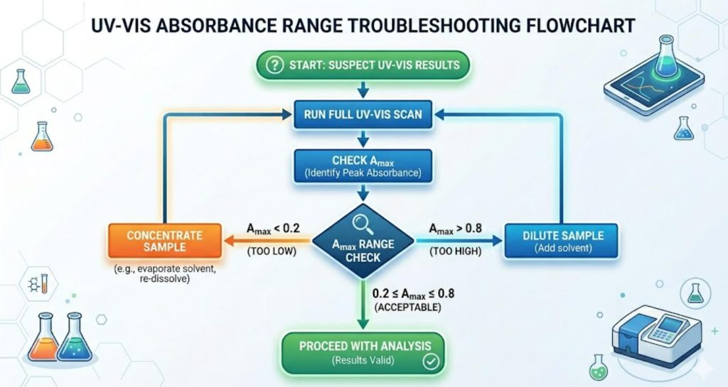
Your sample is telling you what it needs. If a quick spectral scan reveals that the maximum absorbance peak falls outside 0.2–0.8 AU, don’t panic — you have options.

Problem	Symptom	Solution
Too diluted (A < 0.1)	Noisy baseline, unstable readings	Increase concentration (evaporate/centrifuge) or increase path length (use a longer cuvette)
Too concentrated (A > 1.0)	Flat or decreasing signal, suspect calibration	Dilute the sample and remeasure
Moderately high (A > 0.8)	Acceptable but leaving margin for error	Consider slight dilution for safer quantitative work

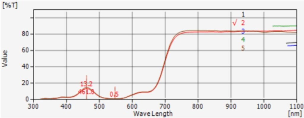
Here’s a practical tip: always run a fullwavelength scan first before you commit to quantitative mode. The scan will show you the maximum absorbance of your sample and its spectral shape — two critical pieces of information that guide every subsequent decision.

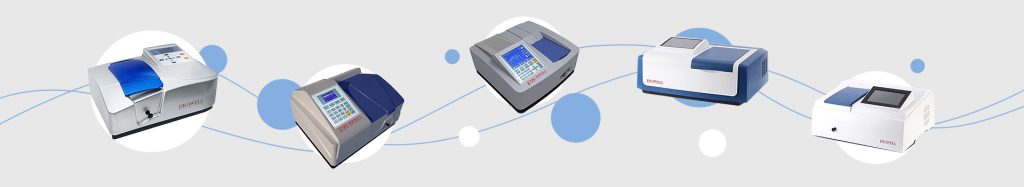
If you have an instrument like Drawell‘s L6 or L7 series UV-Vis spectrophotometers, which support fullspectrum scanning, you can visualize the entire absorbance profile in seconds — no guesswork required.

Case Study: When Absorbance Range Is Wrong

Realworld examples make the principle concrete — and they reveal a pattern worth remembering.

Case 1 — Sample too dilute: An analyst was analyzing samples with absorbance below 0.005 AU on a UVVis instrument with photometric noise around 0.005 AU. Their results were inconsistent and lower than expected. Convinced the instrument was faulty, they called for service. The engineer’s assessment was straightforward: the sample was too diluted. After a modest concentration step, measurements became stable and accurate. The problem wasn’t the instrument — it was operating at the wrong absorbance range.

Case 2 — Sample too concentrated: A researcher was analyzing a food additive, but results consistently ran low — again pointing suspicion at the instrument. A service check confirmed the UVVis spectrophotometer wavelength range was accurate and the optics were clean. The issue? The sample‘s absorbance read 2.5 AU — well above the reliable limit. Upon diluting back to approximately 0.8 AU, repeated measurements delivered highly accurate and reproducible results.

The takeaway? When results look suspicious, don’t assume instrument failure first. Run a quick spectral scan to check your absorbance range. You might save hours of troubleshooting — and avoid costly service calls.

How to Select Spectral Bandwidth (Slit Width)

The 1/10 Rule (FWHM Basis)

When it comes to spectral bandwidth, one principle stands head and shoulders above the rest: set your instrument‘s spectral bandwidth to no more than onetenth of the full width at half maximum (FWHM) of your sample’s absorption peak.

Here’s how it works in practice. First, locate your sample’s main absorption peak in a spectral scan. Measure the peak‘s width at half of its maximum absorbance. That’s the FWHM. Then, set your instrument‘s spectral bandwidth (or slit width, depending on your instrument‘s design) to ≤ 1/10 of that FWHM value.

Why does this work? The spectral bandwidth of a spectrophotometer is defined as the FWHM of the light exiting its monochromator. When the bandwidth is set to 1/10 or less of the sample peak‘s halfwidth, the measurement error is typically within 0.5% [7].

ASTM E95813(2021) provides formalized procedures for estimating spectral bandwidth in the 185 nm to 820 nm region, applicable to all modern spectrophotometer designs [8].

Fixed vs. Variable Bandwidth Instruments

Not all spectrometers are created equal — this matters because it directly affects your bandwidth selection capability.

Instrument Type	Bandwidth Control	Best For
Fixed bandwidth (e.g., photodiode array instruments)	Single setting (often 1 nm, 2 nm, or 4 nm)	Routine QC, samples with broad peaks, labs that value simplicity
Variable bandwidth (gratingbased with adjustable slits)	Selectable across a range (e.g., 0.5 nm to 5 nm)	Method development, samples with sharp peaks, research

The Drawell UVVis spectrophotometer family covers both scenarios. Models like the L3 (1.8 nm fixed) or 752N (2 nm fixed) offer reliable fixedbandwidth options — perfect for laboratories running standard methods every day. For method development and more demanding applications, instruments with selectable bandwidth — such as the DU8200 (4 nm / 2 nm selectable) — provide the flexibility to optimize for different sample types.

Tradeoff: Resolution vs. SignaltoNoise

Choosing a spectral bandwidth is rarely straightforward — because what’s good for resolution is often bad for signal strength. And vice versa.

• Narrow bandwidth (≤ 1 nm): You‘ll see fine spectral detail, clearly separate closelying peaks, and achieve highprecision wavelength accuracy. But less light means higher noise levels — a problem when measuring lowabsorbance samples or when speed matters, as longer integration times may be needed to build signal.
• Wide bandwidth (2 – 5 nm): More light reaches the detector, giving you stronger signals and better sensitivity for quantitation. But wider bandwidth may merge closelyspaced peaks and can reduce measurement accuracy if the peak shape is sharp [4].

So how do you decide? Start by asking two questions: (1) What’s the sharpness of my analyte‘s absorption peak? (2) Do I need to resolve fine structure, or am I mainly quantifying total concentration? For routine quantitative analysis, a bandwidth of 2 nm works well for most samples. For analytes with very sharp peaks (e.g., gasphase spectra), you’ll want 1 nm or even 0.5 nm bandwidth. For samples with broad, featureless absorption bands, 4 nm bandwidth will deliver strong, smooth signals.

How to Experimentally Determine Optimal SBW

Enough theory — let’s get practical. Here‘s a handson method to find the best bandwidth for your sample.

Step 1 — Prepare your sample at a concentration that gives a maximum absorbance around 0.6 AU (the middle of that comfortable 0.2–0.8 window).

Step 2 — Scan across a range of bandwidths. On a variablebandwidth instrument, run successive scans at different SBW settings — 0.5 nm, 1 nm, 2 nm, 4 nm, etc.

Step 3 — Compare the resulting spectra.

What You See	What It Means	Recommended SBW
Peak absorbance decreases as SBW widens	Bandwidth is merging fine structure; true absorbance underestimated	Use narrower SBW
Spectrum shape becomes noisy at narrow SBW	Low light level causing excess noise	Use wider SBW
Spectrum shape is stable and peaks are wellresolved	You‘ve found the sweet spot	That’s your SBW

Step 4 — For verification, prepare a calibration curve at the chosen SBW. If linearity (R² ≥ 0.999) holds across your desired concentration range, you‘ve successfully optimized your method.

Drawell‘s L6S and L7 series UV-Vis spectrophotometers support fullspectrum scanning and can aid in this SBW optimization process.

StepbyStep Selection Workflow for Routine Analysis

Let’s tie it all together. Here’s a distilled workflow you can follow every time you sit down at your UVVis instrument — whether it‘s from Drawell or any other brand. Bookmark this. Print it out. Tape it above your instrument.

Step	Action	What to Check
1	Run a fullwavelength scan of your sample (suitably diluted)	Identify λmax (peak wavelength) and measure its absorbance
2	Check λmax absorbance value	If outside 0.2–0.8 AU, adjust concentration or path length
3	Determine FWHM of the absorption peak (width at halfheight)	This tells you the peak‘s natural sharpness
4	Set your instrument’s spectral bandwidth (SBW) to ≤ FWHM/10	If your instrument has fixed SBW (e.g., 2 nm), be sure the FWHM/10 guideline still holds
5	Build a calibration curve across your intended concentration range	Verify linearity (R² ≥ 0.999) and that measurements stay within 0.2–0.8 AU
6	Run quality control standards and blanks	Document to meet USP <857> or internal SOP requirements

That‘s it. Six steps that take maybe 15 minutes the first time — and five minutes once your method is locked in. Always keep these steps visible for every method development session.

Common Mistakes to Avoid

Everyone makes mistakes — even experienced analysts. The key is catching them before they affect your data. Here are the five traps that catch most users off guard:

1. ❌ Jumping straight to quantification without a full scan.

You wouldn’t drive a car without looking at the road, so why run quantitative analysis without checking the full absorbance spectrum? Scans take seconds and can save hours. Example: one analyst discovered a setup error causing low response after extensive troubleshooting — a quick scan at the start would have immediately revealed the issue.

2. ❌ Diluting a sample to bring its absorbance “into range,” but then dividing the result incorrectly.

This is surprisingly common. The math is simple: measured concentration after dilution × dilution factor = actual concentration. But in the rush of the lab, the step gets forgotten. Doublecheck your calculations.

3. ❌ Using a fixed 1 nm or 2 nm bandwidth for every single sample without question.

Different samples have different spectral characteristics. A 2 nm bandwidth may work perfectly for broad protein peaks but can cause nonlinearity or peak flattening when measuring sharper absorption bands. Always consider whether the sample demands a narrower or wider bandwidth. Better yet — derive the bandwidth you need directly from the FWHM you measured.

4. ❌ Ignoring sample temperature fluctuations and solvent effects.

Temperature affects absorption band shapes, shifts λmax, and can influence baseline stability. USP <1857> specifically includes new sections on temperature coefficients and solvent selection effects for this reason [9].

5. ❌ Assuming instrument failure before checking your settings.

This is the big one — and the most expensive mistake. The two case studies we covered earlier show how often “instrument problems” turn out to be usercorrectable parameter issues. Before calling for service, run through absorbance range and bandwidth one more time.

Frequently Asked Questions (FAQ)

Q1: What is the most accurate absorbance range for UVVis?

A: The theoretical minimum error occurs near 0.434 AU, depending on noise type [1]. For routine work, the safe and widely accepted range is 0.2–0.8 AU, as recommended in practice by USP <857> [3].

Q2: Can I use absorbance values above 1.0 AU?

A: Possibly — but proceed with caution. The limit depends on your instrument’s stray light level. If stray light is below 0.01 %T, measurements up to 3 AU may be feasible [2]. In general, however, keeping absorbance ≤ 1.0 AU avoids straylightinduced nonlinearity. For highabsorbance samples, dilution is the safer path.

Q3: How do I know if my spectral bandwidth is too wide?

A: Compare spectra at different bandwidths. If the peak absorbance decreases as SBW increases, your bandwidth is merging fine structure and underestimating true absorbance. If adjacent peaks appear to merge, the SBW is excessively wide.

Q4: Is the 1/10 rule always necessary?

A: It’s a robust guideline from wellestablished practice. For quantitative analysis with broad peaks, 1/5 may still be acceptable — but the error will be larger. For highresolution applications where spectral shape matters, adhere to the 1/10 rule [7].

Q5: What’s the difference between fixed and variable bandwidth instruments?

A: Fixedbandwidth instruments have a single, unchangeable SBW (e.g., 2 nm on our Drawell 752N). Variablebandwidth instruments allow you to adjust SBW across a range (like the Drawell DU8600R series with selectable bandwidth). Choose fixed for routine, established methods; variable for method development and maximum flexibility.

Q6: How can I check my instrument‘s performance to USP <857> standards?

A: Follow the qualified procedures for wavelength accuracy, absorbance accuracy, stray light, and resolution. Using certified reference materials (CRMs) is preferred over labprepared solutions [3]. For practical guidance, our application specialists can help design a verification protocol tailored to your instrument.

Q7: Does pathlength affect both absorbance range and bandwidth considerations?

A: Yes — but differently for each. Pathlength directly scales measured absorbance: halving the pathlength halves the absorbance, moving a highabsorbance sample into the optimal 0.2–0.8 AU window without changing concentration. This approach preserves sample integrity while improving range compliance. For bandwidth, pathlength is independent; narrow bands may require longer pathlengths to compensate for reduced light throughput. We recommend checking both ranges and bandwidth recommendations simultaneously — scanning a dilution series at your target SBW typically resolves both parameters.

Q8: Does your instrument support variable bandwidth?

A: Yes. Drawell provides both fixedbandwidth models (e.g., L3S Series at 1.8 nm, L8 at 2 nm) and selectablebandwidth models (e.g., DV8200 with 4 nm / 2 nm). Our experts can help you choose the right configuration for your applications — just reach out using the form above or via email.

Need More Help? Talk to Our Specialists

Sometimes guidelines and workflows aren’t enough. If your application pushes the limits — maybe you’re measuring extremely dilute samples near the detection limit, or you need to resolve overlapping peaks in a complex mixture — our technical team is here to help.

Drawell has been supporting analytical laboratories worldwide with robust, affordable UVVis spectrophotometers across a range of configurations: singlebeam and doublebeam, fixed and selectable bandwidth. Perhaps you need help calculating the right absorbance range for your specific sample, or selecting which instrument and bandwidth configuration best matches your method development needs.

Here’s how we can assist:

• Free application consultation — Talk through your sample type, expected absorbance range, and method requirements with a Drawell applications specialist.
• Sample testing support — Send us your test samples; we‘ll run them on a suitable instrument and share results.
• Instrument recommendations — From the L3 and L9 series to the DU8600RN and DWN4S series, we can match a configuration to your application.
• Onsite SOP and validation assistance — We help with setup, IQ/OQ, and method transfer.

Take the next step. → Contact our technical experts directly or request a product quote at [email protected].

��� Reminder — share this guide with a colleague who might benefit from clearer UVVis parameter selection. And when you‘re ready to talk instruments, we’re just a message away.

References

[1] ChemRxiv. Raw Data and Noise in Spectrophotometry. 2024. — Current IUPAC-referenced guidance: limit absorbance to 0.1–1.0 AU; optimal performance at 0.43 AU or 0.86 AU depending on limiting noise type.

[2] Agilent Technologies. Optimum Parameters for UV-Vis Spectroscopy. ICPMS LabRulez. 2021. — Stray light < 0.01% permits measurement up to 3 AU; stray light limits dynamic range.

[3] United States Pharmacopeia. *USP <857> Ultraviolet-Visible Spectroscopy*. — Requirements for wavelength accuracy, absorbance accuracy, stray light limit, and resolution. Harmonized with Ph. Eur. 2.2.25.

[4] Unspecified analytical reference (general knowledge in UV-Vis spectroscopy). — Trade-off between spectral bandwidth, resolution, and signal-to-noise ratio.

[5] Drawell or general lab expert quotation (paraphrased from common UV-Vis educational material). — Bandwidth effect on resolution and sensitivity.

[6] Hellma GmbH & Co. KG. USP<857> (United States Pharmacopeia). Hellma Calibration Standards. — Practical guidance on absorbance range.

[7] JASCO Corporation. *Principles of UV/vis spectroscopy (7) Bandwidth*. JASCO Global. 2020. — SBW defined as FWHM; 1/10 rule; error within 0.5% when SBW ≤ FWHM/10.